Reinforcement Learning with Human Feedback (RLHF): A Comprehensive Deep Dive into Chatbot Fine-Tuning and Beyond

Table of Contents

1. Introduction
   • Motivation
   • What to expect?
2. Quick Intro to the RL Loop
   1. An Intro to Policy Gradient Methods
   2. One instance: PPO
3. Quick Intro to Stages of LLM Model Training
   • Pre-training Phase
   • Optional Supervised Fine-Tuning Phase
   • Motivation for RLHF
   • Details on Reward Modeling
4. Putting Everything Together
   • Mapping RL Terms into Language Generation
   • Mathematical Framework for RLHF
   • Pseudocode

1. Introduction

Motivation

In a world where pre-trained language models like GPT-4 are taking the front seat in natural language processing (NLP) applications, it is essential to understand how these models are fine-tuned to perform specific tasks efficiently. Often, libraries like Hugging Face abstract away the intricate details of this process, leaving users with a gap in knowledge on how exactly these systems work. I am totally grateful that we have such amazing libraries that abstract away all the complicated work. And it would have been impossible for me to grasp the topic if I had not examined their code with a lot of breakpoints :)

Moreover, while several blogs and tutorials introduce the basics of Reinforcement Learning with Human Feedback (RLHF), they rarely go into enough depth or provide a one-to-one mapping of RL concepts to NLP problems. At the end of this post, I will share all the relevant repositories, posts and papers that helped me understand the topic.

This blog aims to fill that gap, giving you an exhaustive look into the RLHF process, particularly in the context of fine-tuning language models like GPT-4. Most importantly, it is a small reward for me, summarizing my adventoruous and torturous learning journey.

What to Expect?

By the end of this article, you should have a strong understanding of how reinforcement learning algorithms, especially Proximal Policy Optimization (PPO), are used in fine-tuning large language models (LLMs). You’ll be taken through the mathematics, the pseudocode, and practical examples to offer a holistic understanding of the topic.

Prerequisites

Unfortunately, this is a little bit of a complex topic marrying methods from RL and NLP. Intermediate level familiarity with RL and NLP and coding makes it easier to understand. Some of the concepts will be kept short for brevity to spare more space of the actual RLHF training loop. I will leave great resources at the end of this post if you think you need to brush up your RL or NLP skills.

Big Picture

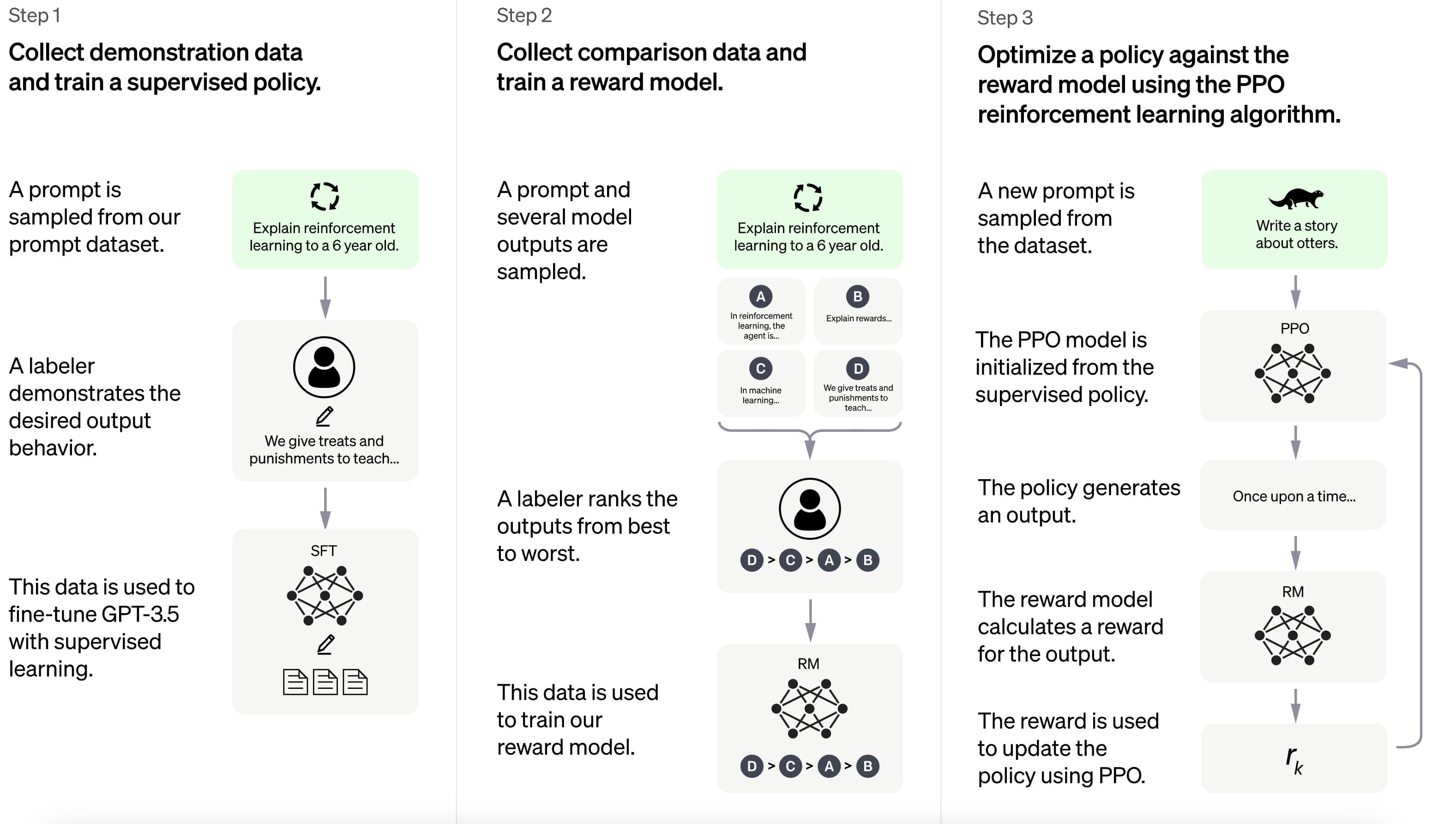
It all starts with a pretrained model. So, we need to pretrain a big language model through self-supervised learning. We basically throw billions of texts on the web and let the model train itself by doing next sentence prediction. Now your GPT is ready but it still does not have that “chat” capability. That is, it is yet to align with human preferences.

The next step involves training a reward model that can give a score given a model response to a prompt. This model is required to complete the state-action-reward loop in classic RL. Once we know how to evaluate a model, we can continuously train our agent with an RL-based optimization set-up. So, after obtaining the reward Model, we start our RL learning algorithm:

1. We sample a prompt from our dataset (state)
2. Our model generates a response (action)
3. We obtain the reward via reward model (reward)
4. We update our model parameters to generate better responses next time.

No worries we will go step by step and talk about the whole process in RLHF below. But before that, we need to have a quick recap in RL.

2. Quick Intro to the RL Loop

In traditional reinforcement learning, we have an agent interacting with an environment. The agent performs actions, observes states, and receives rewards. The RL loop essentially consists of the following steps:

• Initialize state ( S )
• Choose an action ( A ) based on the policy ( $\pi$ )
• Take the action, transition to a new state ( S’ )
• Receive a reward ( R )
• Update the policy ( $\pi$ ) based on the reward

To simplify understanding, state is the information to determine what comes next. In a video game setup, you can think it as how agent sees everything, location of the enemies, the terrain, the health status, and so on. Policy is “brain” of the agent. It is a mapping from states to actions. It basically tells what to do in a state. The whole RL rests on reward hypothesis. Imagine life is like a scavenger hunt. The “reward hypothesis” suggests you won’t just sprint to the “Grand Prize”—let’s say, becoming a rock star, or achieving Zen-like inner peace. Nope, you’re more likely to hop from one clue to the next, gathering smaller prizes along the way. Each little win—learning a guitar chord, meditating without falling asleep—gives you a mini-boost, like a snack-sized Snickers for your soul.

It’s like your brain is your life coach, shouting, “You’re doing awesome, keep going!” every time you hit a mini-milestone. Those small rewards fuel you to keep going, like collecting coins in a video game until you level up. So instead of just dreaming about the finish line, you’re actually motivated to complete the tiny steps that eventually get you there. Your brain keeps you in the game by tossing you feel-good confetti every time you make a little progress.

In essence, the “reward hypothesis” is your brain’s clever way of tricking you into adulting by making it feel like a game you actually want to win. So, you’re not just chasing some lofty end-goal; you’re enjoying the ride one prize at a time!

Note that unlike supervised learning, we only have reward signals here. It is as if your teacher tells you nothing but gives some feedback to your solution to the problem. If he is a good one, he might give you multiple signals along the way, but if it is a tough one you can only get a feedback at the very end of the task (usually when the current state becomes the terminal state, aka exitus.) Note that this would be an extremely hard task; however, this is how we train the models in the context of RL. The amazing thing is that these models do anything for rewards and somehow by trial and error million times, they become experts

2.1 An Intro to Policy Gradient Methods

Note that PPO is just a tiny drop in the ocean of RL, please check David Silver’s Intro to RL course to get a full grasp on the topic. Policy Gradient methods directly optimize the policy rather than value function. They make use of the gradient $\nabla J(\theta)$ to update the policy in the direction that increases expected rewards. We want to find an optimal policy that tells us what to do in a given state $s_t$. Once we know how to behave optimally in any state, we can just follow our policy and maximize the rewards, hence obtaining our goals! Therefore we want to learn a function $\pi$ parametrized by $\theta$, $\pi_{\theta}(a,s)$ which gives us the probability of playing action a in state s. You can think about $\theta$ as the knobs of our function and by optimizing $\theta$ we can select the action with highest probability. However, we need to find a way to measure how good our policy is. We can just use the average reward we get from an episode of states and actions. In otherwords, with a gradient-based setup, we can just maximize average expected reward. The central idea is to adjust the policy in the direction that increases the expected return. Mathematically, this is often formulated as: \(\nabla J(\theta) = \mathbb{E}_{\tau \sim \pi_\theta} \left[ \sum_{t=0}^{\infty} \nabla_\theta \log \pi_\theta(a_t|s_t) R(\tau) \right]\)

Where: $\nabla_\theta$ represents the gradient with respect to our policy parameters, $\theta$. $\tau$ symbolizes a trajectory (or episode) which is a sequence of states, actions, and rewards. $R(\tau)$ is the total reward from one trajectory. The expectation ($\mathbb{E}$) averages over all the trajectories produced by our policy.

Though the equation may appear intimidating, its core idea is straightforward: We’re looking for how to best adjust (or “tweak”) our policy parameters to maximize the reward. This adjustment direction is given by the gradient, $\nabla_\theta$. The term $\log \pi_\theta(a_t|s_t)$ signifies the likelihood of taking action $a_t$ given state $s_t$ under our policy. By multiplying this likelihood with $R(\tau)$, we weight the importance of each trajectory by its total reward. In simpler words, the goal is to find a trajectory that gives us the highest reward and adjust our policy parameters to favor such trajectories. Practically, this means we generate some trajectories using our current policy, collect the rewards, and then update our policy based on these rewards. This gradient ascent approach forms the backbone of many policy gradient methods, including Proximal Policy Optimization (PPO). While PPO introduces additional nuances, the central optimization philosophy remains consistent.

2.2: An Instance: PPO

2.2.1 Why PPO is a Good Improvement

PPO refines traditional training methods. Vanilla policy gradients can make large, risky updates, leading to poor model performance. PPO restricts these updates, ensuring they’re not too drastic. This results in more stable training without needing complex techniques or specific settings. It’s efficient, straightforward, and reliable. Imagine teaching a robot to walk. Traditional policy gradient methods might push the robot to take larger and riskier steps if it helps to move faster. PPO, however, would ensure that the robot only takes marginally bigger steps, balancing between speed and risk.

2.2.2 Mathematical Deep Dive into PPO

Proximal Policy Optimization (PPO) primarily employs a clipped objective function. This function aims to prevent drastic divergences between the old and new policies while still optimizing for the expected reward. The function is defined as: \(L^{CLIP}(\theta) = \min \left( r_t(\theta) \hat{A}_t, \text{clip}(r_t(\theta), 1-\epsilon, 1+\epsilon) \hat{A}_t \right)\) Here, $r_t(\theta)$, or the ratio, represents $\frac{\pi_{\theta}(a_{t}|s_{t})}{\pi_{\theta_{old}}(a_{t}|s_{t})}$. To intuitively understand this, consider the scenario where action $a$ is highly beneficial in state $s_t$. Say, under the current policy, $\pi_{\theta}(a_{t}|s_{t})$ is quite probable with a value of 0.8, but under the old policy, $\pi_{old}$, it’s much less likely with a probability of 0.1. This leads to a high value for $r_t$ (in this case, 8). In such situations, the objective becomes clipped, negating the need for gradient updates. This is because the current policy already offers good action choices, and any changes at this point might be too extreme. However, when $r_{t}$ is confined within the range $[1-\epsilon, 1+\epsilon]$, gradient updates are performed.

The term we haven’t delved into yet is $\hat{A}_t$, the advantage function. It essentially denotes the value of selecting action $a$ in state $s$, relative to the average value of that state. For now, let’s primarily focus on understanding the core of PPO. We will delve deeper into the comprehensive PPO optimization in upcoming sections, where we will elucidate the concept of advantages and critics further.

The typical training procedure for PPO is as follows:

# init buffer
observations = []
rewards = []
actions = []
advantages = []

# Collect data for each step
for each step from 0 to num_steps:
    
    # Get observations for the current step
    
    # Get action and log probability using the current policy (without updating weights)
    action, oldlogprob = agent.get_action_logprob(current_observation)
    
    # Execute the action in the environment and get the next observation and reward
    next_observation, reward, done = environment.step(action)

    # store observation, return
    observations[step] = current_observation
    rewards[step] = reward
    actions[step] = actions

# Compute advtanges for each step
advantages = calculate_advantages(rewards)

# Flatten the batch data
Prepare data for optimization by reshaping observations, actions, advtanges, etc.

# Policy optimization
for each epoch from 0 to update_epochs:
    
    Shuffle batch indices
    
    for each minibatch from the batch:
        
        # Get new log probability using the updated policy
        newlogprob = agent.get_new_logprob(minibatch_observation, minibatch_action)
        
        # Calculate the ratio of the new and old policy probabilities
        ratio = exp(newlogprob - oldlogprob)
        
        # Compute policy loss using clipped objective
        pg_loss = Calculate policy gradient loss using the ratio and advantages
        
        # Update the agent's policy
        optimizer.zero_gradients()
        pg_loss.backward()
        optimizer.step()

It’s natural to wonder about the distinction between old and new policies in this context. Initially, there’s just one parametrized policy—a neural network whose parameters we aim to optimize. tThe “old” policy refers to the policy before the update, and the “new” policy indicates the policy after the update. The algorithm ensures stable training by using a clipping mechanism when calculating the policy loss, preventing overly large policy updates.

In PPO, understanding the value of taking a certain action in a given state is pivotal. This leads us to the concept of advantage, denoted as $A_t$. To compute the advantage, we need a measure of the direct benefit of an action, as well as the expected, average value of the current state. This is where the Critic comes into play.

The Critic is essentially another neural network dedicated to estimating the value of a given state. Think of it as the evaluator or judge that assesses how valuable a particular state might be in terms of expected future rewards. The parameters of the Critic are also trained and refined using gradient descent. However, its primary objective is slightly different: the Critic seeks to accurately predict state values.

Given that the value of a state represents the anticipated cumulative reward from that point onwards, we can use the estimated returns as the “ground truth” for the state’s value. Concurrently, the Critic provides us with its own value estimates, which act as predictions. Discrepancies between these two can indicate how well (or poorly) our Critic is performing.

This sets the stage for the optimization process in PPO, where the key components revolve around these principles:

• Policy Optimization: Using the clipped objective function and advantages to optimize the policy parameters.
• Value Estimation: Training the Critic to improve its state value predictions.
• By balancing these components, PPO aims to both refine its action-taking strategy (via the policy) and improve its understanding of state values (via the Critic).

2.2.3 Combining Proximal Policy Optimization (PPO) Losses

2.2.3.1 Clipped Objective Function

Given the policy $\pi$ our neural network producing the policy, let’s use $\pi_{\theta}$ as the policy with parameters $\theta$ and $\pi_{\theta_{old}}$ as the old policy before the update. The ratio of these policies given an action $a$ and a state $s$ is:

The PPO clipped objective function is:

Where:

• $A_t$ is the advantage estimate of the action at timestep $t$
• $\epsilon$ is a hyperparameter (typically around 0.2) which defines the extent to which the policy can be updated in one step.

2.2.3.2 Value Prediction Loss

For the value function $V(s)$, the squared-error loss is used:

Here, $V_{\text{target}}$ is the estimated value of the state (often using returns or discounted returns).

2.2.3.3. Entropy Bonus

The entropy of the policy is added to encourage exploration:

The entropy bonus is added to the policy objective with a coefficient ( \beta ):

When training agents using reinforcement learning, one of the primary challenges is to balance between exploration (trying out new actions to discover their effects) and exploitation (leveraging known actions that maximize rewards). A common pitfall for many RL agents is getting stuck in a local optimum, essentially repeating actions that seem beneficial in the short term without ever exploring potentially more rewarding alternatives. This is where the concept of entropy comes in as a potential solution.

In the context of PPO and other policy optimization algorithms, the policy (often represented as a probability distribution over actions) has an associated entropy. Mathematically, entropy measures the randomness or unpredictability of this distribution. A uniform distribution, where all actions are equally likely, has the highest entropy, while a deterministic policy, which always chooses a specific action in a given state, has an entropy of zero.

Intuition

The idea behind adding an entropy bonus to the objective function in PPO is to encourage the policy to be more random (explorative) rather than deterministic (exploitative). By doing this, we give the agent an incentive to explore a diverse range of actions, especially in the early stages of training. As training progresses and the agent becomes more knowledgeable about the environment, the entropy of the policy will naturally decrease as the agent learns to exploit the best actions.

Benefits

The entropy bonus helps in multiple ways:

1. Avoiding Premature Convergence: The agent is discouraged from settling on a sub-optimal policy too quickly.
2. Enhanced Exploration: Especially useful in complex environments where the globally optimal strategy might be non-intuitive or hidden.
3. Stabilized Training: Encouraging exploration can also lead to more stable and robust learning, as the agent gets a more comprehensive understanding of the environment.

In summary, the entropy bonus in PPO serves as a regularization mechanism, promoting a healthier balance between exploration and exploitation, and ensuring that the agent doesn’t overlook potentially beneficial strategies.

2.2.3.4 Putting It All Together

Combining all the above terms:

Here, $\alpha$ is a coefficient that determines the weight of the value function loss in the total loss.

The following is a simple pseudocode in python that is more granular than the previous one:

for update in range(num_updates):
    
    # Collect data for num_steps
    for step in range(num_steps):
        obs[step] = next_obs
        action, logprob, _, value = agent.get_action_and_value(next_obs)
        values[step] = value
        actions[step] = action
        logprobs[step] = logprob
        
        next_obs, reward = envs.step(action)
        rewards[step] = reward

    # Calculate returns and advantages
    advantages = torch.zeros_like(rewards)
    for t in reversed(range(num_steps)):
        delta = rewards[t] + gamma * values[t + 1] - values[t]
        advantages[t] = delta + gamma * gae_lambda * advantages[t + 1]
    returns = advantages + values
    
    # Optimization phase
    for epoch in range(update_epochs):
        for minibatch in generate_minibatches():
            _, newlogprob, entropy, newvalue = agent.get_action_and_value(minibatch.obs, minibatch.actions)
            logratio = newlogprob - minibatch.logprobs
            ratio = logratio.exp()

            # Calculate policy loss
            pg_loss1 = -minibatch.advantages * ratio
            pg_loss2 = -minibatch.advantages * torch.clamp(ratio, 1 - clip_coef, 1 + clip_coef)
            pg_loss = torch.max(pg_loss1, pg_loss2).mean()

            # Calculate value loss
            v_loss = 0.5 * ((newvalue - minibatch.returns) ** 2).mean()

            # Combine losses
            loss = pg_loss - ent_coef * entropy.mean() + v_loss * vf_coef
            
            # Update agent
            optimizer.zero_grad()
            loss.backward()
            optimizer.step()

Now that we understood the basics of PPO. We can continue with RLFH, our ultimate goal!

3. Quick Intro to Stages of LLM Model Training

Pre-training Phase

LLMs are usually first trained on a large dataset in an unsupervised manner. This dataset is a mix of everything: from books to Wikipedia pages, from forum discussions to tweets. In general, this is a noisy text. However, the main goal is to teach the model the internals of the language. This can be regarded as the general knowledge. However, a pretrained model cannot be used as a chatbot right away. If we want to have something that is inline with our preferences, we need to further finetune the model. That is why, we need the following steps.

Optional Supervised Fine-Tuning Phase

After pre-training, the models can be optionally fine-tuned using a labeled dataset. OpenAI, hires plenty of contractors to generate high quality datasets in the form of <prompt, response>. The main goal is to further train the model in the same format but on a high quality dataset. Note that for RLHF, this step is not mandatory. Feel free to skip this one if you don’t have enough budget. Or you can use some heuristics such as DeepMind to generate high-quality dataset from the existing data on the web.

Reward Modeling

Remember in PPO, we need a way to evaluate how good an action is. In LLM context, we need to find a way to evaluate a response given a prompt. And this evaluation should be in line with human preferences. Reward Modeling comes to the rescue. Before RLHF, we train a separate model called reward model (RM) that returns a scalar value given prompt and response. This model is usually a clone of the pretrained model with a modified head so that it just returns a scalar value. OpenAI, achieves it by creating a dataset of tuples <prompt, winning_response, losing_response>. Basically, for a prompt sampled from the dataset, finetuned model(s) generate multiple responses and labelers rank those responses as winner and loser. Given a prompt, winning response and losing response model is trained with a pairwise ranking loss. specifically utilizing the log-sigmoid of the difference between the scores of the winning and losing responses. This loss ensures that the score for the winning response is higher than the score for the losing response by maximizing the difference between the two scores.

Let $s_w$ is the score for the winning response and $s_l$ is one for losing. We minimize \(-E_{x \in D}[\log(\text{sigmoid}(s_w - s_l))]\) where $x$ is the response distributed over the dataset we collected. After training our reward model, we can easily generate a score for a text response, so apply our reinforcement algorithm on our LLM.

RLHF

Understanding RLHF is easy once we have a good understanding of PPO. Let’s try to map what we learned in the previous section to the NLP context. Think about every step or state transition as facing a new token.

In RL, we switch from state s to s’ while in NLP, it is switching from “Hello” to “Hello, I”. At a high level, the text we have so far represents our current state while the next word choice represents our action. So action is a choice from the vocabulary defined by our tokenizer. By chosing a token (word), we directly append it to our current state so that our current state becomes “Hello, I, #chosen-token3” RLHF in language models mainly involves training the model to optimize the expected reward $E[s]$, using similar objective functions as used in PPO. The reward is easy, it is coming from our reward model. score, $s$ is obtained by $RM(prompt, response)$. This is a sparse reward setting in classical RL. Although you generate many tokens, till the end, you will be getting 0 reward. Only when you reach your terminal state with ‘EOS Token’, the response is put into our reward model and our reward for the whole sequence is obtained.

One might ask, what about our critic here? Do we have any value function to compute the advantages? Yes, in HuggingFace (HF) library, the current language model is modified to have a separate ‘ValueHead’ that calculates value of a state.

Here the excerpt from the HuggingFace’s TRL library

class ValueHead(nn.Module):
    r"""
    The ValueHead class implements a head for GPT2 that returns a scalar for each output token.
    """

    def __init__(self, config, **kwargs):
        super().__init__()
        if not hasattr(config, "summary_dropout_prob"):
            summary_dropout_prob = kwargs.pop("summary_dropout_prob", 0.1)
        else:
            summary_dropout_prob = config.summary_dropout_prob

        self.dropout = nn.Dropout(summary_dropout_prob) if summary_dropout_prob else nn.Identity()

        # some models such as OPT have a projection layer before the word embeddings - e.g. OPT-350m
        if hasattr(config, "word_embed_proj_dim"):
            hidden_size = config.word_embed_proj_dim
        else:
            hidden_size = config.hidden_size

        self.summary = nn.Linear(hidden_size, 1)

        self.flatten = nn.Flatten()

    def forward(self, hidden_states):
        output = self.dropout(hidden_states)

        # For now force upcast in fp32 if needed. Let's keep the
        # output in fp32 for numerical stability.
        if output.dtype != self.summary.weight.dtype:
            output = output.to(self.summary.weight.dtype)

        output = self.summary(output)
        return output

Remember when we feed the language model with an input, we have the hidden states for every step. Therefore, we can easily calculate the value of each state thanks to this ValueHead. For the rest of this blog, I will base my code reference to TRL library and explain their PPO training code.

RLHF Training

We also use an additional reference model, which can be the pretrained model. Apart from all the PPO loss discussed above, we want to regularize our loss function with KL divergence score that measures the choice of actions between two models (distributions in general.). In other words, we will penalize our model if it diverges or deviates too much from the reference model. This is to ensure that our model does not learn to hack the RL reward by producing gibberish but still getting a good reward.

Now we have everything needed. The training loop has the following idea. We sample a prompt and generate response by our model. Then we get the score by the reward model then update our model parameters. Then sample new prompt and so on. In the next section we go line by line over the TRL library code to fully grasp each step. Note that we will just work on a single prompt to understand what is going on. Feel free to play with more prompts and batches.

So, we initialize the model to be trained and the reference model

# init models
model = AutoModelForCausalLMWithValueHead.from_pretrained('gpt2')
ref_model = create_reference_model(model)
# init reward model
reward_model = RewardModel("gpt2")
# init tokenizer
tokenizer = AutoTokenizer.from_pretrained('gpt2')
tokenizer.pad_token = tokenizer.eos_token

# set PPO config
ppo_config = PPOConfig(
    batch_size=1,
)

# encode a query
query_txt = "This morning I went to the "
query_tensor = tokenizer.encode(query_txt, return_tensors="pt")

# get model response
response_tensor  = respond_to_batch(model, query_tensor)

# create a ppo trainer
ppo_trainer = PPOTrainer(ppo_config, model, model_ref, tokenizer)

# initialize a random query
reward = reward_model.predict([query_tensor, response_tensor])

# train model for one step with ppo
train_stats = ppo_trainer.step([query_tensor[0]], [response_tensor[0]], reward)

The step code is a pseudo-code that shows the basic flow and hide many implementation details. Please visit TRL library and put actual debbugger points to actually check all the details from normalizations to input validation to masking.

I did not mention logprobabilities

def step(queries, responses, scores, model, ref_model):
    # scale and clip the score (reward)
    scores = score_and_clip(scores)
    with torch.no_grad():
        # do a forward pass to obtain log_probabilities
        # note that we obtain the values by the ValueHead of the model!
        logprobs, values, masks = forward_pass(model, queries, responses)
        # do a forward pass with ref model
        ref_logprobs, _, _ = forward_pass(ref_model, queries, responses)
        # compute rewards here and subtract kl penalty from the score
        # kl penalty is a metric of shape [seq_length] showing the difference between two responses
        # so we calculate kl score for every position in the sequence
        kl = kl_penalty(logprobs, ref_logprobs)
        # note that score is also for every position but as discussed it is zero for all the previous steps. It is non-zero at the last position
        rewards = scores.clone() - kl_coefficient * kl
        # just remember that while reward is 0 except the last step, kl can have non zero values at each step
        # now we can calculate advantages just like we did before
        advantages = compute_advantages(values, rewards)

        # this was our "play" stage, now we will go over our batch many times and update our model parameters
        for _ in range(ppo_epochs):
            for _ in range(mini_batch_update_step):
                # do a forward pass with the minibatch
                mini_logprobs, mini_values = batched_forward_pass(model, queries, responses)
                # select what we calculated before as 'old'
                old_logprobs = batch["logprobs"][mini_batch_inds]
                # select the previously calculated values
                old_values = batch["values"][mini_batch_inds]
                # returns are required to calculate value prediction error
                returns = batch["returns"][mini_batch_inds]
                # in the next session we will calculate the losses
                # in this specific implementation value predictions are also clipped 
                vpredclipped = clip(mini_values, old_values, clip_delta)
                value_loss = calculate_value_loss(vpredclipped, returns)
                # then we calculate the action probability ratios this is required to calculate policy loss
                # again ratio is of shape [mini_batch_size, sequence_length] 
                # because we compare the action probabilities per position in the response
                ratio = torch.exp(mini_logprobs - old_logprobs)
                policy_loss_unclipped = -advantages * ratio
                policy_loss_clipped = -advantages * torch.clamp(ratio, 1 - cliprange, 1 +cliprange)
                # take the max of both (note that in maximization we take the min as described in the blog)
                # note pg_loss is calculated for every step (position in the sequency)
                # that is why at the end we average over the response length
                # note masks are omitted for brevity but they are required so that the prompt or context
                # is not used for calculation policy_loss
                policiy_loss = torch.max(policy_loss_unclipped, policy_loss_clipped).mean()
                # note that in TRL loss calculation, I could not find the addition of entropy to the loss function
                # although it is being calculated.
                loss = policy_loss + value_coefficient * value_loss
                # backpropogation and update gradients
                loss.backward()
                optimizer.step()
                optimizer.zero_grad()

Voila! Now we can train our own LM with RLHF. This concludes my blog. I think this is a very complex training procedure although I tried to hide many implementation details in the actual code. Please don’t try to implement your own as it is very easy to make mistakes. I suggest using those off-the-shelf libraries such as TRL library. Also, after spending many hours understanding RLHF, there is one bad news for you. Recent research found easier finetuning method bypassing the RL in human preference alignment. This new method is called DPO(Direct Preference Optimization). According to the research, this method gives better results than tuning with PPO. The good news is that, this new method has been derived from RLHF. So, once you have a good understanding in it, it will be very easy to understand the latter.

Resources

1. Chip Hyen’s blog on RLHF
2. Huggingface StackLlama
3. Hugging Face RLHF
4. HF RLHF topic
5. Instruct GPT
6. Stiennon (2020), Learning to Summarize from HF
7. Self-instruct Paper
8. TRL Library